I recently bought the novel ‘The Bell Jar’ by Sylvia Plath. This came about as follows. I have now lived in Mainz for over ten years. Bookshops exert a strong attraction on me. It is therefore strange that I had never entered the shop ‘Shakespeare and so …’ which I must have passed very many times. Now I have done so. I had nothing special in mind and I had no definite plan to buy anything. I spent quite some time looking around the shelves and in the end I did buy a book, ‘The Bell Jar’ by Sylvia Plath. I knew the title of the book and the name of the author but not much more than that. So why did I feel attracted to it? I guess that it is due to the fact that forty years ago Ali Smith talked to me positively about the author. I do not know if this is really the case but it seems to me plausible. I suppose that the recommendation has slumbered in my unconscious all the time and was brought out again by the chance encounter with the book. I did once have a flat-mate who was writing a PhD on Ted Hughes, the husband of Sylvia Plath, but I do not think that the recommendation came from him. In fact I must have read at least one poem by Plath at that time since on the way home the following fragment which must have been lodged in my memory came into my mind: ‘ebon in the hedges fat’. After I got home I was able to find out that it comes from a poem called ‘Blackberrying’, which must have impressed me as a student. On the way home in the tram I read the first few pages of the novel and it became clear to me that it was a piece of luck that I had bought the book. I had the delicious experience of beginning to read a book and immediately feeling at home.
Reading the book was a positive experience for me from beginning to end, although it includes things I experienced as frightening perspectives. I had warm feelings towards both the protagonist and the author. The book has now been given a place of honour on the bookshelf containing those books I esteem most. I do not feel that I have to provide a justification for the feelings I have just expressed but I will at least mention a couple of aspects of the book which have played a role in producing these. One is the remarkable objectivity with which Plath describes all kinds of things which in principle could have a strong emotional impact. Here I think of Jünger although the authors’ subjects are so different. A second is the way I experience many of Plath’s sentences. When the sentence starts you think it is going in a certain direction and then it suddenly turns and goes in quite a different one. A third is the fact that the book presents a picture of mental illness as seen from the inside. Here I think of the shell-shocked veteran in Mrs Dalloway who I see as portraying some part of Virginia Woolf’s illness. A fourth is that I was struck by the fact that the main character assesses the attractiveness of men by the sound of their names. I never proceeded in this way when deciding how attractive I found women but in this point, where in a sense language overrules reality, and in several others in the book I felt ‘This could be me’. As a last point I simply mention the great originality of the book which is quite different from any other book I have read. This originality is not just an effect of the book as whole but instead impregnates the whole text.
 in terms of derivatives of
  . In fact we will only write out those terms explicitly which do not always vanish at the bifurcation point. The result is
  .
. . Note, however, that the expression
  is not intrinsic to the centre manifold. Because of the vanishing of the first derivatives the second order derivatives
  and
and  define tensors in the full dimension of the dynamical system. Hence we can write
  invariantly in the form
  . It remains to compute
  . The invariance of the centre manifold implies that
  . Hence
  . This equation has a unique solution for
  . In this way one of the conditions for a generic cusp bifurcation can be expressed in an invariant way. This corresponds to (8.128) in the book of Kuznetsov. In trying to understand these things better I was confused by equation (5.28) in the book which should be almost the same as (8.128) but in fact contains a typo. There is a repetition of
  . For a generic cusp bifurcation we need two parameters
  and
and  . The genericity condition involving derivatives with respect to parameters can easily translated into an invariant form. The result is
 Formulae similar to those just given were used in a paper I wrote with Juliette Hell some years ago (Nonlin. Analysis: RWA. 24, 175). Looking back at that I have the feeling that we must have been doing some sleepwalking when writing that paper. Or maybe I was sleepwalking and Juliette was paying attention. In any case, the final result was correct.
 and a steady state
  . The usual aim is to understand systems up to certain transformations. One type of transformation is of the form
  . A second is of the form
  . A third is of the form
  . With the assumptions which have been made we can do a translation to achieve
  . Assume now that the linearization of the system at the origin is diagonalizable with rank one. Then it has one eigenvalue zero and one non-zero eigenvalue. It can be diagonalized by a linear transformation of the coordinates. After these transformations the system has almost been reduced to the form in the last post, except that there is a non-zero constant in front of the first summand in the evolution equation for
  which might not be
  . It can be reduced to the latter case by rescaling the time coordinate. A similar process can be carried out when the centre manifold is of higher codimension. Then the variable
  for an invertible matrix
  . The function
  defining the centre manifold is then also vector-valued. The centre manifold analysis can be done in a manner very similar to what we have seen already.
 and its derivatives with respect to
  unchanged. The derivative of
  is rescaled by the non-zero factor
  and so the fact of its being non-zero is unchanged. The third type of transformation just scales all the relevant quantities by the non-zero factor
  and so also does not change whether these are zero or not. It remains to consider the second type of transformation. At this point a more geometrical point of view will be adopted. We change the notation for the right hand side of the equations to
  . These are the components of a parameter-dependent vector field which satisfies
  . Because of this condition the derivative
  defines a vector at the origin independently of the transformation of the second type. The linearization
  of the vector field at the origin defines a tensor. We suppose as before that it is diagonalizable and of rank one. Let
  be a vector spanning the kernel of
  . Similarly there is a one-form
  with
with  . It is unique up to rescaling and we choose it to satisfy
  . With these notations the condition previously written in the form
  can be written in the invariant form
  . The condition previously written in the form
  can be written in the invariant form
  . Here we use the notation
  . It is because the vector field vanishes at the origin and
  and
and  . This example is general enough to illustrate several important ideas. Here
  are supposed to be smooth and vanish at least quadratically near the origin. The linearization of this system has the eigenvalues
  . It follows that there exists a centre manifold of the form
  , where
  . Substituting this into the evolution equation for
  . This is a leading order approximation to the flow on the centre manifold. If
  we can use it to read off the stability of the origin within the centre manifold. This argument uses no information about the way the centre manifold deviates from the centre subspace, i.e. how fast
  we need to go further.
 . Call this equation (*). It can be analysed with the help of the Taylor expansions
  and
and  . Substituting these into (*) we see that the left hand side is of order three. Thus the same must be true of the right hand side and we get
  and
and  . Substituting this back into the evolution equation for
  . Thus if
  . If it is zero we can do another loop of the same kind. Looking at the third order terms in the equation (*) we get
  . This allows the fourth order term in the evolution equation for
  in the equation for
  . If it is non-zero we are done. If it is zero use the equation (*) to determine the leading term in the expansion of the centre manifold. Put this information into the equation for
  and
and  , where
  . The origin is a steady state of the extended system and the centre manifold at that point is of dimension two. It is of the form
  . Suppose that we are in the case
  . Of course the equation
  remains unchanged. We can now check the conditions for a generic fold bifurcation in the system reduced to the centre manifold. The first is
  . The second is
  . Hence
  is equivalent to
  . The third involves
  . We see that
  is equivalent to
  . The fourth involves
  . We see that
  is equivalent to
  ,
,  . The functions
  are defined on
  where
where  is a bounded domain in
  with smooth boundary. Let the
  be denoted collectively by
  . I assume that the diffusion coefficients
  are non-negative. If some of them are zero then the system is degenerate. In particular there is an ODE special case where all
  for all
  . It should then follow that in the presence of suitable boundary conditions
  for all
  . I assume that
  and
and  it follows that
  . (This means that if a chemical species is not present it cannot be consumed in any reaction.) It turns out that this condition is enough to ensure positivity.
 on the interval
  where
where  and
and  are continuous functions with
  and suppose that
  . I claim that
  for all
 ![t^*=\sup\{t_1:u(t)\ge 0\ {\rm on}\ [0,t_1]\}](https://s0.wp.com/latex.php?latex=t%5E%2A%3D%5Csup%5C%7Bt_1%3Au%28t%29%5Cge+0%5C+%7B%5Crm+on%7D%5C+%5B0%2Ct_1%5D%5C%7D&bg=ffffff&fg=333333&s=0&c=20201002) . Since
. Since  . Assume that
  . By continuity
  . If
. If  were greater than zero then by continuity it would also be positive for
  slightly larger than
  , contradicting the definition of
  . The evolution equation then implies that
  . This implies that
  for
for  and this completes the proof of the desired result.
 and
and  . We would like to conclude that
  for positive constants
  and
and  . Then
  . Hence
 ![\dot v=-au+[b+\epsilon\sigma e^{\sigma t}]](https://s0.wp.com/latex.php?latex=%5Cdot+v%3D-au%2B%5Bb%2B%5Cepsilon%5Csigma+e%5E%7B%5Csigma+t%7D%5D&bg=ffffff&fg=333333&s=0&c=20201002) and
and  . Now
. Now  and so
 ![\dot v=-av+[b+\epsilon(\sigma+a) e^{\sigma t}]](https://s0.wp.com/latex.php?latex=%5Cdot+v%3D-av%2B%5Bb%2B%5Cepsilon%28%5Csigma%2Ba%29+e%5E%7B%5Csigma+t%7D%5D&bg=ffffff&fg=333333&s=0&c=20201002) . It follows that if
. It follows that if  satisfies the conditions satisfied by
  for all
  on
on  . It also involves approximating non-negative data by positive data. A difference is that the proof just given does not use the continuous dependence of solutions of an ODE on initial data and in that sense it is more elementary. In Theorem 3 of the paper of Mincheva and Siegel the former proof is extended to a case involving a system of PDE.
 and a boundary condition
  . Here
  is that in the direction of the outward unit normal to the boundary. We assume that
  and a
and a  extension to
  . We now replace the differential equation by the differential inequality
  . We assume that the initial data are non-negative,
  . The assumption that
  . The aim is to show that all solutions of the resulting system of inequalities are non-negative. We assume the condition for a system of chemical reactions already mentioned.
 is strictly positive on
  . We define
 ![[0,t_1]](https://s0.wp.com/latex.php?latex=%5B0%2Ct_1%5D&bg=ffffff&fg=333333&s=0&c=20201002) is the longest interval where the solution is non-negative. We suppose that
is the longest interval where the solution is non-negative. We suppose that  with
with  and
and  for all
  . Suppose first that
  . Then
  and
and  . This contradicts the strict inequality related to the evolution equation for
  is on the boundary of
  and
and  . This contradicts the strict inequality related to the boundary condition for
 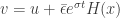 . Here
  is the vector all of whose components are
  is a positive function. It is obvious that
  . We now choose
  which ensures its positivity and require that the outward normal derivative of
  on the boundary is equal to one. (Here I will take for granted that a function
 ![\frac{\partial v_i}{\partial t}-d_i\Delta v_i-f_i(v)\ge e^{\sigma t}\epsilon[\sigma H-d_i\Delta H-L\sqrt{n}H]](https://s0.wp.com/latex.php?latex=%5Cfrac%7B%5Cpartial+v_i%7D%7B%5Cpartial+t%7D-d_i%5CDelta+v_i-f_i%28v%29%5Cge+e%5E%7B%5Csigma+t%7D%5Cepsilon%5B%5Csigma+H-d_i%5CDelta+H-L%5Csqrt%7Bn%7DH%5D&bg=ffffff&fg=333333&s=0&c=20201002) where
where  is a Lipschitz constant for
  and, letting
  , that